Explaining base rate neglect
In a seminar for a team from an investment manager I described how base rates are often neglected when people are grappling with conditional probabilities. My description was somewhat confusing, so the below is a short write-up for the participants.
–
Consider the following question scenario.
You test yourself with a rapid antigen test for COVID-19. The following information is known:
- The probability that a person has COVID-19 is 1% (the prevalence).
- If a person has COVID-19, the probability that they test positive using this brand of rapid antigen test is 90% (the sensitivity).
- If a person does not have COVID-19, the probability that they nevertheless test positive is 9% (the false positive rate).
You test positive. What is the chance that you have COVID-19?
When students, doctors and other experimental subjects answer variants of this question, a common response is around 80% to 90%.
Yet, the answer is approximately 9%. There are far more false positives than true positives. For those that are mathematically inclined, this is a fairly simple application of Bayes’ rule (shown in the Appendix below).
The correct answer becomes more apparent if I show an alternative representation, such as the following:
You test yourself with a rapid antigen test for COVID-19. The following information is known:
- Ten in every 1000 people have COVID-19 (the prevalence)
- Of these 10 people with COVID-19, nine will test positive (the sensitivity)
- Of the 990 people without COVID-19, about 89 nevertheless test positive (the false positive rate).
You test positive. What is the chance that you have COVID-19?
This use of natural frequencies was first proposed by Cosmides and Tooby (1996) (pdf). Natural frequencies are derived from observing cases that have been representatively sampled from a population.
In a paper by Gigerenzer and Ulrich Hoffrage, they report that this change in representation increased the proportion of correct answers among physicians from 10% to 46%.
There is some evidence (e.g.) that you can get further gains through a frequency tree representation. Here’s one such tree from Gigerenzer (2011), which also has the benefit of further highlighting the benefits of the natural frequency approach.
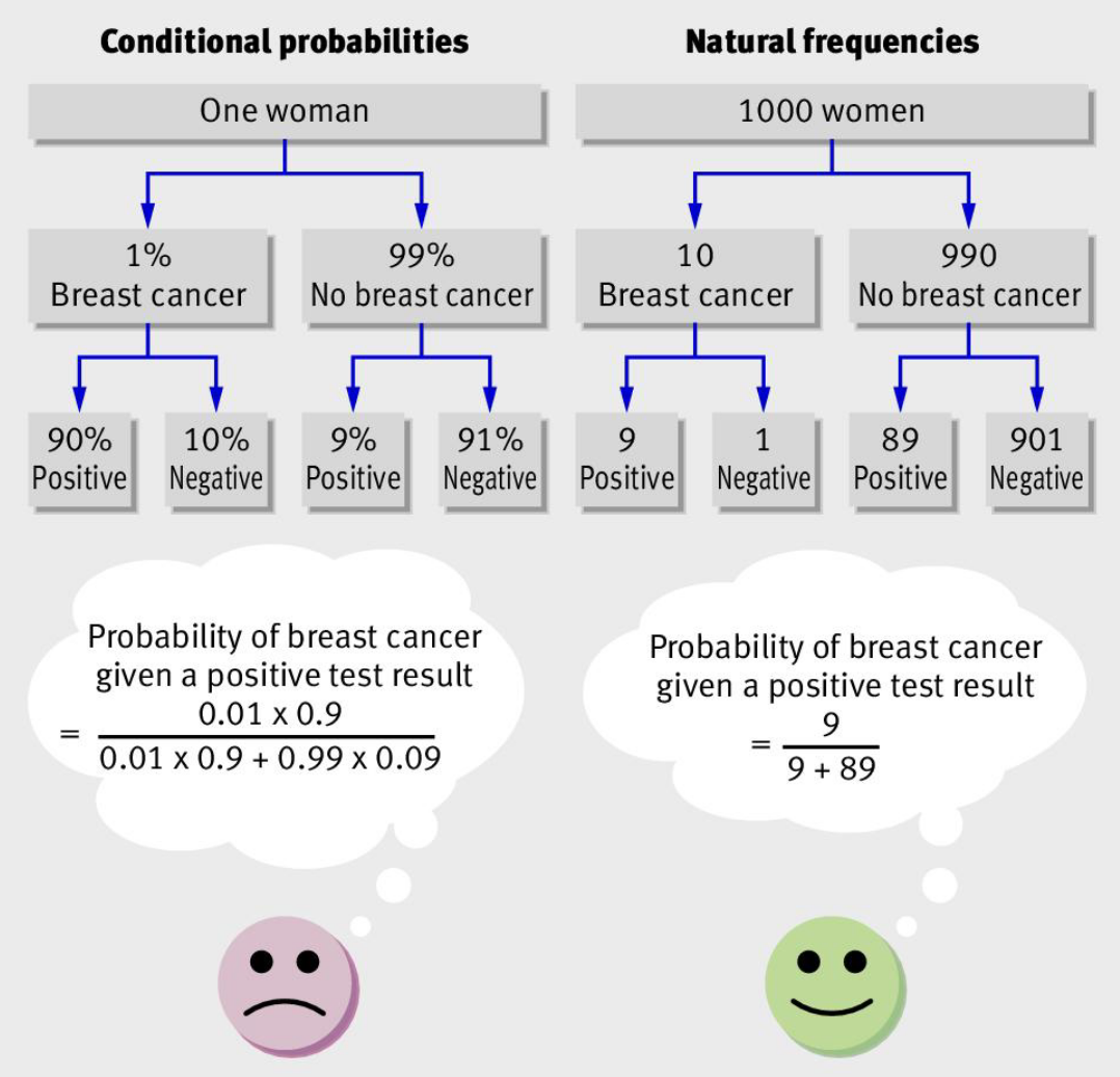
The numbers at the bottom of the conditional probability tree do not contain the base rate information. You can’t simply compare across them in calculating conditional probabilities. You also need to refer back to the middle layer. Conversely, the natural frequency tree contains all you need in the bottom row.
Note that we could convert the numbers in the bottom of the conditional probability tree into frequencies: 900 in 1000, 10 in 1000, 90 in 1000 and 910 in 1000. Gigerenzer calls these simple frequencies.
There are many scenarios where simple frequencies can make a problem more tractable, but they do not solve the computational complexity here. Simple frequencies are just a restatement of the probabilities. In contrast, natural frequencies are joint frequencies, such as the number of people who test positive and who have COVID-19.
So why do people make errors of the type described above in the first place?
One explanation is that people confuse the conditional probability of having COVID-19 given a positive test with the conditional probability of receiving a positive result given they have COVID. That is, they confuse P(COVID-19 | positive) with P(positive | COVID-19).
This mistake leads to the largest errors when the base rate of the event you are attempting to predict - in this case having COVID-19 - is low. Confusing the two conditional probabilities effectively results in the base rate being neglected.
Another explanation is that there are two types of information here: general information in the form of a base rate and specific information in the form of a positive test. The positive test is representative of a person who has COVID-19, so is given greater weight than the more general information.
Let’s now put this classic problem into a domain relevant to you.
You want to know if management of a company or managed fund is skilled. You want to know this as you believe skilled management can lead to outperformance. The following (completely made up) information is known:
- 10% of managers or management teams are skilled.
- If a management team is skilled, the probability that they outperform the market is 90%.
- If a management team is unskilled, the probability that they outperform the market is 40%.
You observe an outperforming firm or fund. What is the probability that they are skilled?
It’s not 90%. We are not asking the probability of outperformance if they are skilled.
For this example we have a higher base rate than for the COVID-19 example: 10% of teams are skilled. But the evidence on performance has a weaker link to skill than a positive test does to COVID-19. 40% of unskilled teams outperform. There are many false positives.
The result: 20% of outperforming teams are skilled. There is some signal in the noise, but it is weak signal. You cannot neglect that low base rate of skilled teams.
Mathematical appendix
Applying Bayes’ rule to the COVID diagnosis:
\begin{align*} P(\text{COVID | positive}) &=\dfrac{P(\text{positive | COVID})P(\text{COVID})}{P(\text{positive})} \\[12pt] &=\dfrac{P(\text{positive | COVID})P(\text{COVID})}{\Bigg(\begin{align*} P&(\text{positive | COVID})P(\text{COVID}) \\ &+P(\text{positive | not COVID})P(\text{not COVID}) \end{align*}\Bigg)} \\[30pt] &=\dfrac{0.9\times0.01}{0.01\times0.9+0.99\times0.09} \\[12pt] &=0.092 \end{align*}Applying Bayes’ rule to the assessment of skill:
\begin{align*} P(\text{skill | outperform}) &=\dfrac{P(\text{outperform | skill})P(\text{skill})}{P(\text{outperform})} \\[12pt] &=\dfrac{P(\text{outperform | skill})P(\text{skill})}{\Bigg(\begin{align*} P(&\text{outperform | skill})P(\text{skill}) \\ &+P(\text{outperform | no skill})P(\text{no skill}) \end{align*}\Bigg)} \\[30pt] &=\dfrac{0.9\times0.1}{0.9\times0.1+0.4\times0.9} \\[12pt] &=0.2 \end{align*}